Computational Simulation

Goal: estimate a causal effect when you do not have data from a randomized experiment
Strategy 1: Re-weighting each observation by the probability of receiving A or B so that the data approximates a randomized experiment
Strategy 2: Modelling the outcome directly with a linear regression
Combining Idea 1 and 2: To form doubly robust estimator

Setting up data

We assign \(X_1\) and \(X_2\) as causal variables, and define a true ACE of 10.

simu_observational_data <- function(simu_id = 1, n_obs) {
  X_1    <- rnorm(n_obs)
  X_2    <- rnorm(n_obs)
  XB     <- 0.2*X_1 + 0.2*X_2
  prob_A <- exp(XB) / (1 + exp(XB))
  A      <- rbinom(n_obs, 1, prob_A)
 
  # We set the true causal effect of treatment A is 10
  Y      <- 100 + X_1 + 2*X_2 + 10*A + rnorm(n_obs)
 
  # summarize variables into a data frame
  data.frame(simu_id = simu_id, n_obs = n_obs,
             var_1 = X_1, var_2 = X_2,
             treatment = A, outcome = Y)  
}

n_simu <- 150
n_obs <- 200

set.seed(1)

data <-
  purrr::map2_dfr(1:n_simu, rep(n_obs, n_simu), simu_observational_data) %>%
  group_by(simu_id)

sl.lib <- c("SL.mean","SL.glm")

IPW model

We create the correct model of IPW with both variables, \(X_1\) and \(X_2\).

prop_score_model <- function(data) {
  glm(treatment ~ var_1 + var_2, data = data, family = 'binomial')
}

#IPW estimator is correct
ipw_estimator <- function(data, model) {
  data %>%
    mutate(
      prob = predict(model, newdata = data, type = 'response'),
    ) %>%
    summarise(
      # Calculate expected value for both treatment and non-treatment using IPW equation
      EY0_ipw = mean(outcome*(1 - treatment) / (1 - prob)),
      EY1_ipw = mean(outcome*treatment / prob)
    ) %>%
    # Calculate ACE
    mutate(ipw = EY1_ipw - EY0_ipw)
}

We miss \(X_2\) in the model, which makes the model misspecified.

prop_score_model_w <- function(data) {
  # OOPS! I forgot var_2
  glm(treatment ~ var_1, data = data, family = 'binomial')
}

# IPW estimator is wrong
ipw_estimator_w <- function(data, model) {
  data %>%
    mutate(
      prob = predict(model, newdata = data, type = 'response'),
    ) %>%
    summarise(
      # Calculate expected value for both treatment and non-treatment using IPW equation
      EYB_ipw = mean(outcome*(1 - treatment) / (1 - prob)),
      EYA_ipw = mean(outcome*treatment / prob)
    ) %>%
    # Calculate ACE
    mutate(ipw_w = EYA_ipw - EYB_ipw)
}

REG model

We create the correct model of outcome regression model with both variables, \(X_1\) and \(X_2\).

mean_outcome_model <- function(data) {
  glm(outcome ~ treatment + var_1 + var_2, data = data)
}

#REG estimator is correct
outcome_model_estimator <- function(data) {
   mean_model <- mean_outcome_model(data) # Compute the model
   summary(mean_model)$coefficients['treatment', ][1] # Coefficient for treatment
}

We miss \(X_2\) in this model, which makes this REG model misspecified.

mean_outcome_model_w <- function(data) {
  # MISSING var_2??!?!
  glm(outcome ~ var_1 + treatment, data = data)
}

# REG estimator is wrong
outcome_model_estimator_w <- function(data) {
   mean_model <- mean_outcome_model_w(data) # Compute the model
   summary(mean_model)$coefficients['treatment', ][1] # Coefficient for treatment
}

Data Simulation

We build the data with all different model specifications.

n_simu <- 150
n_obs <- 200

set.seed(1)

nested_df <-
  purrr::map2_dfr(1:n_simu, rep(n_obs, n_simu), simu_observational_data) %>%
  group_by(simu_id) %>%
  nest() %>%
  mutate(
    # correct ipw model
    prop_model     = map(data, prop_score_model),
    # incorrect ipw model
    prop_model_w   = map(data, prop_score_model_w),
    # correct reg model
    mean_model     = map(data, mean_outcome_model),
    # incorrect reg model
    mean_model_w   = map(data, mean_outcome_model_w),
    # correct reg estimation
    model_estimate = map(data, outcome_model_estimator),
    # incorrect reg estimation
    model_estimate_w = map(data, outcome_model_estimator_w),
    # correct ipw estimation
    ipw_estimate   = map2(data, prop_model, ipw_estimator),
    # incorrect ipw estimation
    ipw_estimate_w = map2(data, prop_model_w, ipw_estimator_w),
  ) %>%
  ungroup() %>%
  unnest(c(model_estimate, model_estimate_w, ipw_estimate, ipw_estimate_w))

Now, we have five models: IPW (both correct and incorrect), REG (both correct and incorrect), and DRE.

Strategy 1: Inverse Probability Weighting (IPW)

Intuition Behind it

In an experiment the probability of receiving a treatment are always equal across all units (50%)
In the current case, the probability of receiving the treatment depends on variables that affect the outcome
If we knew what this probabilities are we could re-weight our sample such that the data would better match a randomized experiment - by creating the “pesudopopulation” (mentioned earlier)
Reminder: propensity score is just a logistic regression of the probability of receiving the treatment, giving their \(Z\) values (confounders)

In our example, we proposed the correct IPW model:

prop_score_model <- function(data) {
  glm(treatment ~ var_1 + var_2, data = data, family = 'binomial')
}

Introducing IPW estimator

Similar to a difference of means but weights each observation inversely proportional to its probability of receiving a treatment (propensity score \(\widehat {PS_i}\))

\[\hat{\delta}_{IPW} = \frac{1}{n}\sum_{i=1}^{n}\bigg[\frac{E[Y_{i}|{A=1}]}{\color{red}{\widehat {PS_i}}} - \frac{E[Y_{i}|{A=0}]}{\color{red}{1-\widehat {PS_i}}}\bigg]\]

Generating IPW estimator and calculate ACE by IPW equation:

ipw_estimator <- function(data, model) {
  data %>%
    mutate(
      prob = predict(model, newdata = data, type = 'response'),
    ) %>%
    summarise(
      EY0_ipw = mean(outcome*(1 - treatment) / (1 - prob)),
      EY1_ipw = mean(outcome*treatment / prob)
    ) %>%
    mutate(ipw = EY1_ipw - EY0_ipw)
}

IPW Performance

Plot for correct IPW

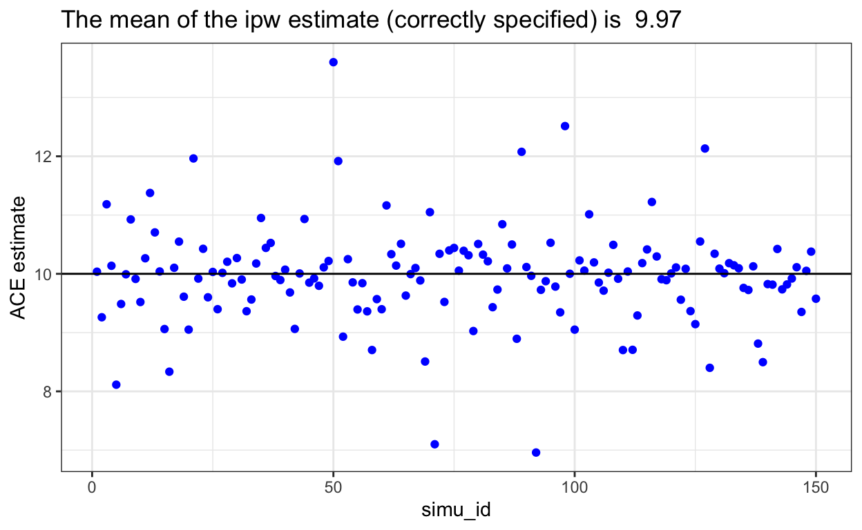
The plot shows the data points are evenly spread around 10, and the mean of correct IPW estimate is 10, which is very close to the true ACE we set.

IPW could fail

If the model for A is incorrect, it would cause bias in the IPW, which cause IPW to fail. We used the biased ipw results from the ‘nested_df’ dataset.

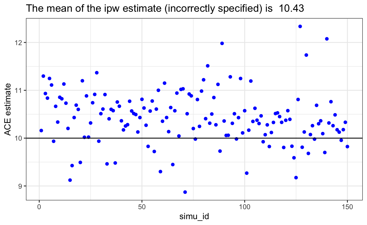
The plot shows a obvious trend that all data points from biased IPW model shift upward, which the ACE for incorrect IPW model is higher than the ACE=10 we set in the beginning.

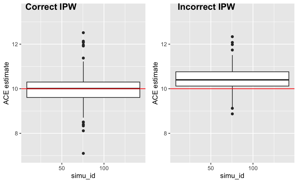
We overestimated the true ACE (which is 10) if we wrongly specified the model form in IPW setting.

Strategy 2: REG estimator (model the outcome)

outcome_model_estimator <- function(data) {
   mean_model <- mean_outcome_model(data)
   summary(mean_model)$coefficients['treatment', ][1]
}

REG Performance

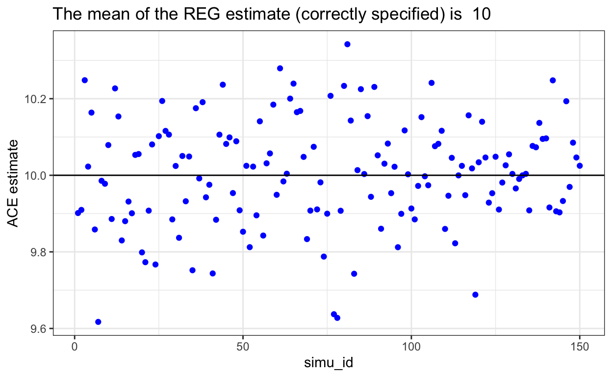
When outcome model is correctly modelled, this shows unbiased estimation of ACE.

REG could also fail

If the model for Y is incorrect (as we recalled we left var_2 out), it will cause bias in the REG outcome model, which cause the model to fail.

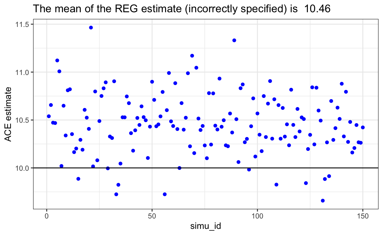
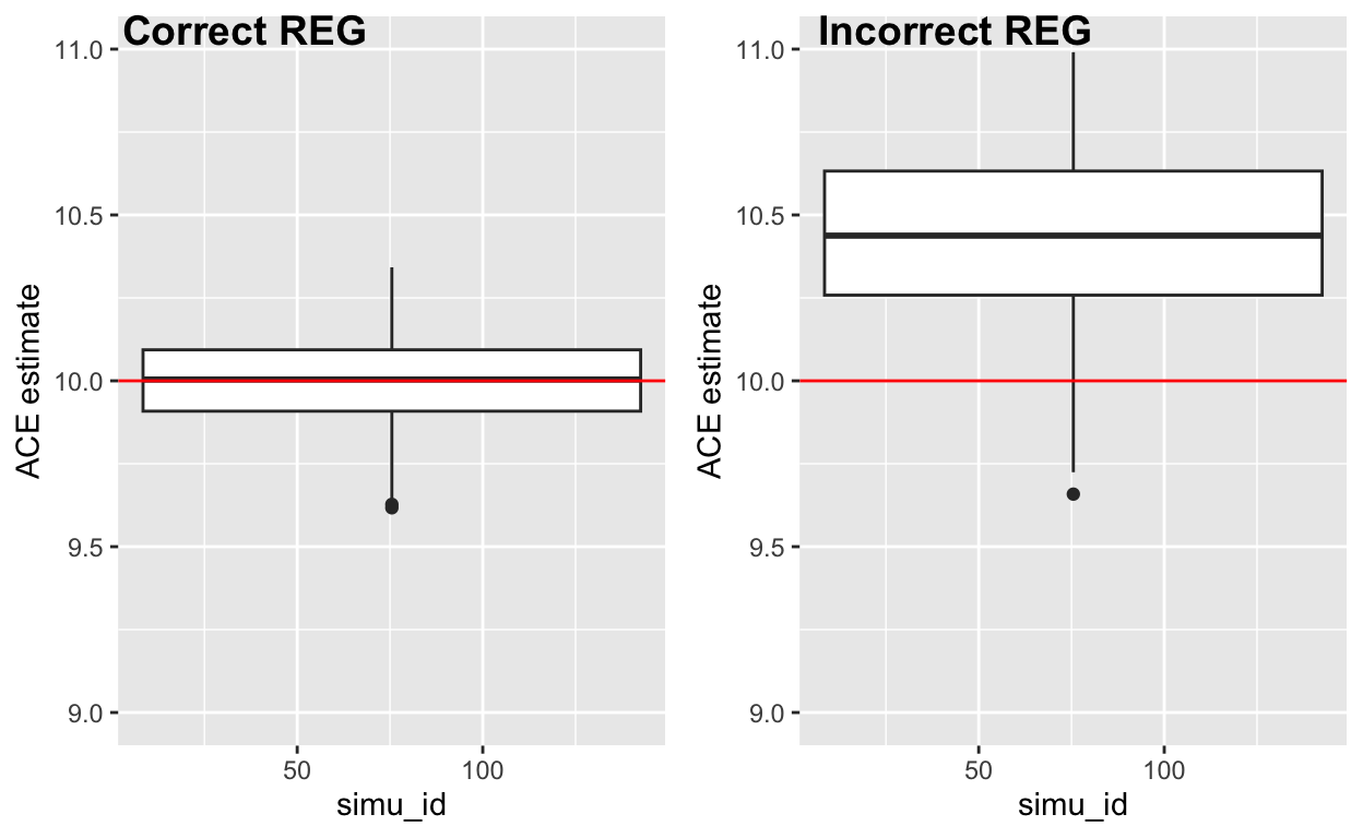
We also overestimated the true ACE (10) if our REG model is mis-specified.

Combining Strategy 1 and 2

If the propensity score model is incorrect, strategy 1 will not work
If the outcome model is incorrect, strategy 2 will not work
If you combine both approaches, you just need either one to work but not both
This is “doubly robust” property!

Doubly Robust Estimator

DRE’s estimation of average causal effect can be summarized into this equation (it is the same thing as the one in the previous section but we changed some notations):

\[\hat{\delta}_{DRE} = \frac{1}{n}\sum_{i=1}^{n}\bigg[\frac{Y_{i}A_{i} -\color{red}{(A_i-\pi(Z_{i}))\mu(Z_i, A_i)}}{\pi(Z_{i})} - \frac{Y_{i}(1-A_{i}) -\color{red}{(A_i-\pi(Z_{i}))\mu(Z_i, A_i)}}{1-\pi(Z_{i})}\bigg]\]

where \(\pi(Z_i)=\widehat {PS_i}\) (propensity score from IPW), and \(\mu(Z_i, A_i)=E[Y|A=1,Z]\) (this is the part of outcome regression model in DRE model). The term in red is said to augment the IPW estimator.

When IPW and REG both correct

AIPW_00 <- AIPW$new(Y= data$outcome, 
                    A= data$treatment,
                    W= subset(data,select=c(var_1,var_2)), # Covariates for both IPW and REG models
                    Q.SL.library = sl.lib, # Algorithms used for the outcome model (Q).
                    g.SL.library = sl.lib, # Algorithms used for the exposure model (g).
                    k_split = 10, # Number of folds for splitting
                    verbose=FALSE)
AIPW_00$fit()
# Estimate the average causal effects
AIPW_00$summary(g.bound = 0.25)
dre_00 <- AIPW_00$estimates$risk_A1[1] - AIPW_00$estimates$risk_A0[1] # Calculate ACE
dre_00

Estimate 
10.00317

This is fine - we have a very unbiased estimation.

Let’s analyze DRE’s performance under following settings:

When IPW is Incorrect, REG is correct

Let’s explore what happens to DRE when something goes wrong!

AIPW_01 <- AIPW$new(Y= data$outcome,
                    A= data$treatment,
                    W.Q= subset(data,select=c(var_1,var_2)), # Covariates for the REG model.
                    W.g= subset(data,select=var_1), # Covariates for the IPW model.
                    Q.SL.library = sl.lib,
                    g.SL.library = sl.lib,
                    k_split = 10,
                    verbose=FALSE)
AIPW_01$fit()
AIPW_01$summary(g.bound = 0.25)
dre_01 <- AIPW_01$estimates$risk_A1[1] - AIPW_01$estimates$risk_A0[1]
dre_01

Estimate 
 10.0033

The mean of estimates are around 10. This indicates that this estimator is unbiased when IPW is misspecified.

When REG is incorrect, IPW is correct

AIPW_10 <- AIPW$new(Y= data$outcome,
                    A= data$treatment,
                    W.Q= subset(data,select=var_1), 
                    W.g= subset(data,select=c(var_1,var_2)),
                    Q.SL.library = sl.lib,
                    g.SL.library = sl.lib,
                    k_split = 10,
                    verbose=FALSE)
AIPW_10$fit()
AIPW_10$summary(g.bound = 0.25)
dre_10 <- AIPW_10$estimates$risk_A1[1] - AIPW_10$estimates$risk_A0[1]
dre_10

Estimate 
10.00384

The mean of estimates are also around 10. This indicates that this estimator is unbiased when REG is wrongly modeled.

When both REG and IPW are incorrect - DRE fails!!

Let’s look at what happens to DRE estimation when both models are incorrectly identified. From previous slides, we learned how robust DRE is - its unbiasedness holds even if one of the models is incorrect, but this is not the case here!

AIPW_11 <- AIPW$new(Y= data$outcome,
                    A= data$treatment,
                    W.Q= subset(data,select=var_1), 
                    W.g= subset(data,select=var_1),
                    Q.SL.library = sl.lib,
                    g.SL.library = sl.lib,
                    k_split = 10,
                    verbose=FALSE)
AIPW_11$fit()
AIPW_11$summary(g.bound = 0.25)
dre_11 <- AIPW_11$estimates$risk_A1[1] - AIPW_11$estimates$risk_A0[1]
dre_11

Estimate 
 10.4585

The mean of estimates are above 10 (10.46). This indicates that this estimator is biased when both REG and IPW are wrongly modeled.

Looking at them together!

               ACE estimates
Both Correct        10.00317
IPW Incorrect       10.00330
REG Incorrect       10.00384
Both Incorrect      10.45850

Conclusion

This simulation activity shows how effective DRE is - that its effectiveness depends on correct model specification or outcome regression model (REG), or inverse Probability weighting by propensity score (IPW). Its robustness is maintained when one of the models is incorrect.

From previous work, we have also identified and learned why DRE is unbiased when either of them is incorrect. If we have non-randomized trial experiments, we can surely apply methods introduced here today!

Doubly Robust Estimator: simulation activity in R