Gibbs Sampler involves working with conditional distributions - the core of Bayesian ideas. Let’s take a look at Bayesian World and how they are connected.
Background: Bayesian V.S. Frequentist
Frequentist is the dominant philosophy and category in the modern statistical world. In fact, many concepts/ thinking/ logic we have been exposed from statistics are from Frequentist beliefs, such as “confidence interval”, “p-value”, “the true value of an unknown parameter”, etc. However, Gibb’s sampler is a method that applies conditional probability distribution, where the “conditioned” nature indicates its Bayesian flavor. This page serves as a refresher to get a taste of Bayesian Statistics - we will briefly talk about its knowledge building process of estimating unknown parameters, learn Bayes rule, and do a little exercise on deriving the posterior distribution of an unknown parameter.
Unlike Frequentists who deem unknown parameters as unknown, fixed constants, Bayesians think about them as random variables and constantly changing their beliefs about unknown parameters based on the data we truly see - they start by proposing a possible probability distribution for the unknown parameter (prior distribution), and find out what they actually see from real data to update/ change the beliefs by deriving posterior distribution based on the prior distribution and data. Furthermore, by seeing more data, they continue to update their knowledge on the parameter (for example, shrink the parameter space/ support by lowering the plausibility of some values of which the parameter can take).
We can imagine the parameter is a Plasticine or modeling clay. When we buy a Plasticine from a store, it has its original shape (prior - the beginning hypothesis/ information we have about the parameter), and its shape constantly changes corresponding to the external forces applied (data we’ve seen so far). The resulted shapes are the posterior - the information we gained about parameter after seeing data.
The end goal of Bayesian estimation is not to see a convergence and shrinkage of parameter space and determine the most likely value of a parameter- that sounds like “Frequentist”. In Bayesian, we never end updating the knowledge based on data.
Sounds like there is lots of “based on”, “dependent on”, and “after seeing…” in Bayesian - YES, this explains why our topic of Gibbs Sampling is contextualized on Bayesian side - Gibbs sampler involves with working with conditional distributions.
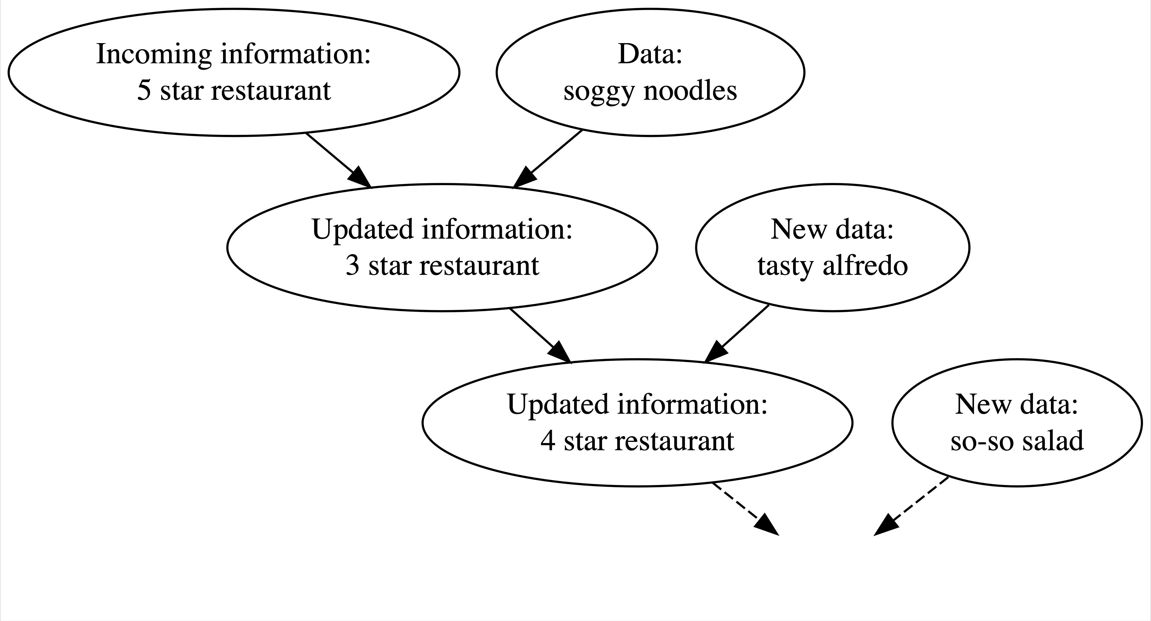
Figure below illustrates Bayesian knowledge-building process: Johnson, A. et.al. If we heard from many 5-star reviews from a restaurant that you are going to visit, we may start expecting it to be a 5-star restaurant.
You sit down, and they serve you a really soggy noodles, you’d be upset and surprised - at the same time, you overthrow your previous assumption about the restaurant and thought it was really just a 3-star level. Then, they serve you a really yummy dish and you change your impression back to 4-star as for now…
Through observing and changing, Bayesians are giving themselves more flexibility of estimating parameters of interest. They do estimations based on “Bayes rule” - a central idea and foundation of Bayesian statistics.
Bayes Rule
Connecting back to probability terms, let’s remind ourselves the Bayes rule of two events \(A\) and \(B\), generalized by equation below:
\[ P(A| B )= \frac{P(A\cap B)} {P(B)}=\frac{P(B|A)P(A)}{P(B)} \]
where:
- \(P(A)\) and \(P(B)\) are the independent probabilities that they happen
- \(P(A\cap B)\) is the probability that both A and B happen
- \(P(B|A)\) is the conditional probability given A happens
By knowing the independent probabilities of \(A\) and \(B\), and seeing the probability of \(B\) happens given A happens, we can derive what do we know about \(A\) given B.
In Bayes, \(A\) will reflect our known parameters, and \(B\) will reflect our data. Let’s take a further step to see how this connects to probability distribution as a whole.
Use Bayes rule in probability distribution
Suppose we are interested in the unknown parameter \(\theta\). How do we update our guess?
First, We start by proposing a prior distribution to the unknown parameter \(\theta\): denote this as \(p(\theta)\) if discrete or \(f(\theta)\) if continuous. For example, if \(\theta\) represents a probability, then one may suggest their prior to be \(\theta \sim Unif(0,1)\). There is no right or wrong/ good or bad judgment calls to priors- they are completely subjective and based on personal knowledge/ background research to the parameter.
Next, we will incorporate our data by calculating the likelihood of seeing a sequence of observations \(\vec{X}\) under \(\theta\): denoted as \(f(\vec{X}|\theta)\).
Thirdly, We are interested in posterior distribution of the parameter - update! Denote this as \(g(\theta|\vec{X})\) to differentiate the updated distribution.
According to the Bayes rule, we can calculate the posterior distribution \(g(\theta|\vec{X})\) by (suppose \(X, \theta\) are both continuous random variables):
\[ g\left(\theta \mid \vec{X} \right) =\frac{f\left(\vec{X} \mid \theta\right) f(\theta)}{f(\vec{X})} \] where \(f\left(\vec{X} \mid \theta\right)\) is the joint pdf/ likelihood given \(\theta\) and the denominator \(f(\vec{X})\) is the marginal pdf of \(\vec{X}\).
Notice that the posterior distribution of \(\theta\) does not depend on \(\vec{X}\), that leads us to a convention in deriving the posterior distribution \(g(\theta \mid \vec{X})\) because we can ignore the actual composition of \(f(\vec{X})\) as it only serves as the normalizing constant in deriving a pdf for a random variable. Therefore:
\[ g\left(\theta \mid \vec{X} \right) \propto {f\left(\vec{X} \mid \theta\right) f(\theta)} \] Note that the pdf of posterior distribution of \(\theta\) is not equal to the right hand side - we still need the marginal pdf of \(\vec{X}\) to calculate the exact pdf. But the above equation gives us the kernels in a pdf - they are sufficient enough to let us find out the posterior distribution of \(\theta\).
Exercise: deriving posterior distribution for \(\theta\)
Let’s try a simple example (from Dr. Kelsey Grinde’s in class material on Bayesian Statistics). Suppose we observed one random observation of a coin flip, \(X\sim Bern(p)\), and we are interested in \(p\), where we assume its prior distribution: \(p \sim Beta (a,b)\). We derive the posterior distribution \(g(p \mid X)\):
\[ \begin{aligned} g(p|X) &\propto f(X\mid p) f(p)\\ &= [p^X (1-p)^{1-X}] \quad [\frac{\Gamma(a+b)}{\Gamma(a)\Gamma(b)} p^{a-1} (1-p)^{b-1}]\\ & \propto p^X(1-p)^{1-X} p^{a-1}(1-p)^{b-1} \\ & =p^{X+a-1}(1-p)^{1-X+b-1} \\ & p \mid X \sim \operatorname{Beta}(X+a, 1-X+b) \\ & \end{aligned} \]
We only conserve terms with \(p\) and dump anything else such as constants \(a, b\). Notice how \(a,b, X\) and the number of trial (1 in this case since we only have one random observation) are incorporated into the posterior distribution.
The example above works with single unknown parameter \(p\), and Gibbs sampling works with Bayesian to obtain posterior samples of multiple unknown parameters (many dimensions). Furthermore, it is noteworthy that Gibbs is only applied to situations when we have multiple unknown parameters and it is hard to calculate the joint, posterior distribution of all parameters using the method above (so we do not have a single posterior distribution, but many - this means we cannot derive i.i.d. samples but dependent samples), and it is easier/ feasible to derive their individual conditional posterior distributions. We will learn about it more on the next page!